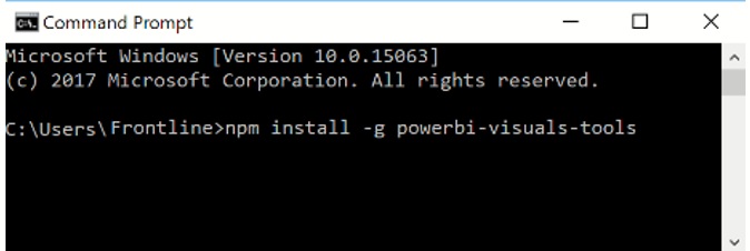
Uploading Your RASON Model to Power BI

Starting with V2019, you can turn your RASON-based model into a Microsoft Power BI Custom Visual. Where others must learn JavaScript (or TypeScript) programming and a whole set of Web development tools to even begin to create a Custom Visual in Power BI, after reading this section, RASON users will be able to create one right away.

To summarize, users simply select rows or columns of data to serve as changeable parameters, then choose Create App – Power BI (on the Editor tab) and save the file created by Rason. Afterwards, users click the Import a Custom Visual icon in Power BI and select the file just saved. What is produced isn’t just a chart – it’s a full optimization or simulation model, ready to accept Power BI data, run on demand on the web and display visual results in Power BI. Users simply need to drag and drop appropriate datasets into the “well” of inputs in Power BI to match the model parameters.

The Rason Server translates the Excel model into RASON® (RESTful Analytic Solver Object Notation, embedded in JSON), then “wraps” a JavaScript-based Custom Visual around the RASON model. See the previous chapter “Creating Your Own Application” for more information on RASON.

Installing Power BI

Power BI is Microsoft’s desktop or cloud-based interactive data visualization business intelligence tool. Starting with V2019, RASON users can turn their Excel based optimization or simulation model into a Microsoft Power BI Custom Visual;that is the full optimization or simulation model, ready to accept Power BI data, run on demand on the web and display visual results in Power BI.

Note: Click this link to download Power BI for desktop.

In order to use this new feature, you must first open desktop Power BI or the free cloud based version of Power BI. (Power BI is part of the office 365 suite.) For more information on this business tool, see the following website.

It is important to note, that in order to create a custom visual in Power BI, you will first need to install Power BI’s Developer Tools which is comprised of NodeJS and the Power BI tools. Follow the steps below to install both required items.

• Click here to download NodeJS.
• Click the Download LTS button to download NodeJS for 64-bit Windows.
• Once the NodeJS installer is downloaded, run the installer and follow the directions on the installer dialogs to install NodeJS onto your machine.
• Install the command line tools by opening a command prompt and typing: “npm install -g powerbi-visuals-tools” as shown in the screenshot below.

After clicking Enter, you’ll see the following results in the command prompt window.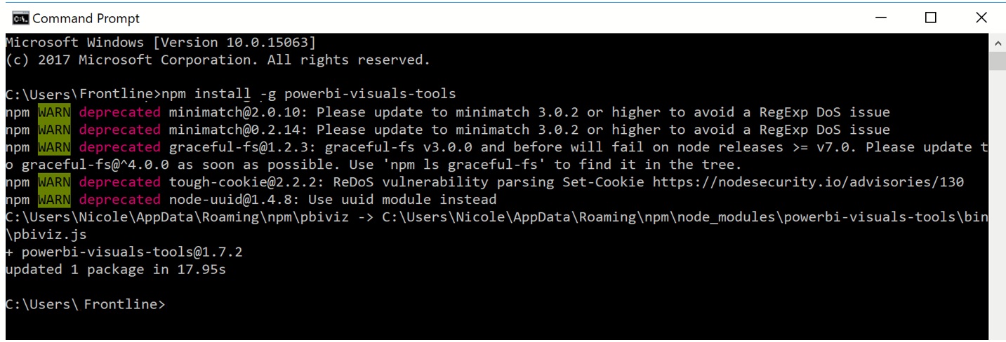

Creating a Custom Visual from a RASON Model

Now that the Developer Tools are installed, we can move on to a small RASON example. In this section, we will create a custom visual using the Product Mix example model.

In this section, we will create a custom visual for Power BI using the Product Mix example model. Log on to www.RASON.com and then click on the Editor tab. Click the Rason Examples folder (on the top right), then click Optimization With Data Binding -- ProductMixCsv4.json from the list. Recall this example model determines the optimal mix of products that a company should produce in order to maximize profits. For a complete description of this model, see the Defining your Optimization Model chapter that appears previously in this guide.

In order to create a Custom Visual for Power BI, your RASON model must be formulated using an index set. The example code below creates two ordered sets, parts and prods. The parts set contains five items (in order as entered): chas, tube, cone, psup and elec while the prods set contains 3 items: tv, stereo and speakers. An indexSet is always defined as a JSON object{}. For more information on index sets, see the Rason Reference Guide.

The example code below uses the dataSources section to create three datasources, parts_data, invent_data and profit_data; using three CSV files. Any supported file type may be used. As discussed in previous sections, a dataSource allows data to be passed to the RASON Server using an external data file in a supported file type. By using an external data file, we can submit updated data to the RASON Server without having to edit our existing RASON model. For example, imagine that Purchasing was able to obtain a discount on Speakers and our inventory increased from 800 to 1,000. If we were not using an external data file, we would have to edit the RASON model directly to reflect this change.

{
    "modelName": "ProductMixCSV4",
    "modelType": "optimization",
    "comment": "Example of using CSV table binding to read params and save results",
    "indexSets": [{
        "name": "parts",
        "value": ["chas", "tube", "cone", "psup", "elec"]
    }, {
        "name": "prods",
        "value": ["tv", "stereo", "speaker"]
    }],
    "datasources": {
        "parts_data": {
            "type": "csv",
            "connection": "ProductMixParts.txt",
            "indexCols": ["parts", "prods"],
            "valueCols": ["qty"]
        },
        "invent_data": {
            "type": "csv",
            "connection": "ProductMixInventory.txt",
            "indexCols": ["parts"],
            "valueCols": ["inventory"]
        },
        "profit_data": {
            "type": "csv",
            "connection": "ProductMixProfits.txt",
            "indexCols": ["prods"],
            "valueCols": ["profits"]
        }
    },
    "data": [{
        "name": "parts2",
        "binding": "parts_data",
        "valueCol": "qty"
    }, {
        "name": "invent",
        "binding": "invent_data",
        "valueCol": "inventory"
    }, {
        "name": "profit",
        "binding": "profit_data",
        "valueCol": "profits"
    }],
    "formulas": [{
        "name": "piv_parts",
        "formula": "PIVOT(parts2, { 'prods' }, { 'parts' })"
    }],
    "variables": {
        "name": "x",
        "dimensions": ["prods"],
        "value": 0,
        "lower": 0,
        "finalValue": [],
        "indexValue": []
    },
    "constraints": [{
        "name": "c",
        "dimensions": ["parts"],
        "formula": "MMULT(piv_parts, x) - invent[]",
        "upper": 0,
        "finalValue": []
    }],
    "objective": {
        "name": "total",
        "formula": "sumproduct(x, profit[])",
        "type": "maximize"
    }
}

DataSources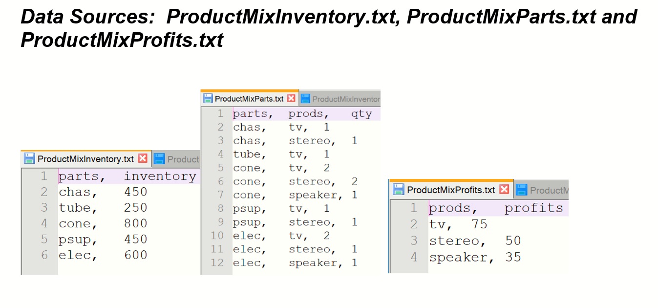

The first data source, parts_data, contains two index columns, parts and products, i.e., a LCD TV requires 2 Electronic components. The next two data sources, invent_data and profit_data, include one indexCol and one valueCol. These two properties create a dataframe. (While properties indexCols and valueCols create a RASON table.) The indexCol is the column containing the indices or the labels and the valueCol is the column containing the values for the indices.

    
  "datasources": {
    "parts_data": {
      "type": "csv",
      "connection": "ProductMixParts.txt",
      "indexCols": [ "parts", "prods" ],
      "valueCols": [ "qty" ],
      "direction": "import"
    },

    "invent_data": {
      "type": "csv",
      "connection": "ProductMixInventory.txt",
      "indexCols": [ "parts" ],
      "valueCols": [ "inventory" ],
      "direction": "import"
    },

    "profit_data": {
      "type": "csv",
      "connection": "ProductMixProfits.txt",
      "indexCols": [ "prods" ],
      "valueCols": [ "profits" ],
      "direction": "import"
    }
  }

Data

In the data section, "profit" is bound to the column "profits" within the data source, "profit_data", "parts2" is bound to the "qty" column within the "parts_data" datasource and "invent" is bound to the "inventory" column within the "invent_data" datasource.

  "data": [
    {
      "name": "parts2",
      "binding": "parts_data",
      "valueCol": "qty"
    },

    {
      "name": "invent",
      "binding": "invent_data",
      "valueCol": "inventory"
    },

    {
      "name": "profit",
      "binding": "profit_data",
      "valueCol": "profits"
    }
  ],

The three variables are specified within variables, the constraints are created within constraints (using a Pivot Table) and the objective is computed and maximized within objective. For more information on using a pivot table within Rason, see the Using Tables section that occurs in the chapter, Using Array Formulas, For Loops and Tables in Rason.

Click Create App – Power BI to create the Power BI custom visual. Save the custom visual in a location of your choice.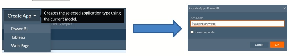

Open either desktop or cloud-based Power BI. The screenshot below depicts the opening screen of desktop Power BI. Click the icon containing three horizontal dots that appears at the bottom of Visualizations (in the top right-hand corner).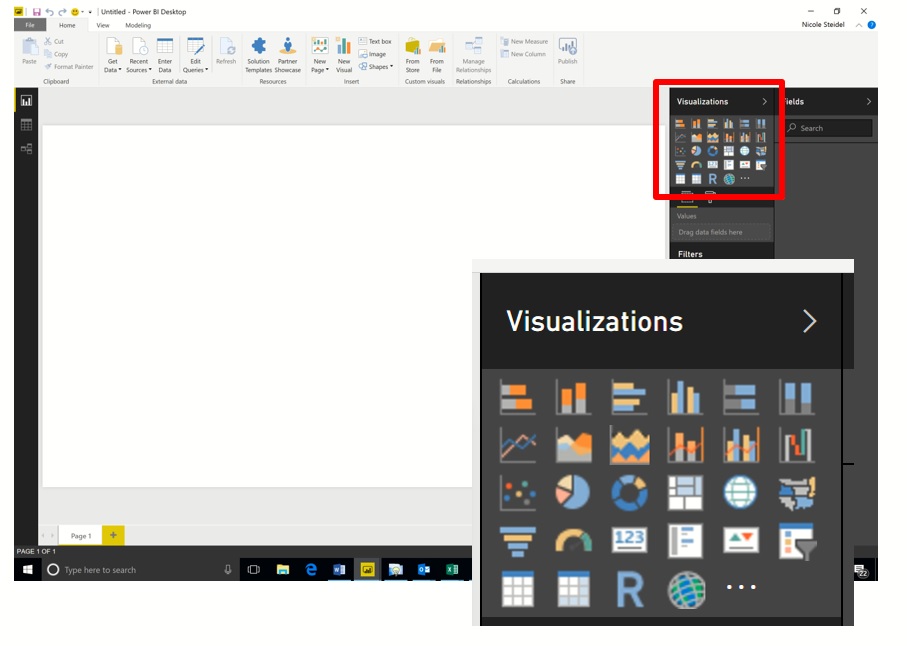

Then select Import from file from the menu.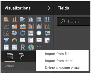

Click Import on the Import custom visual dialog that appears. (You can select Don’t show this dialog again if you’d rather not see this dialog each time you import a custom visual.)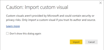

Navigate to the location of the saved Power BI custom visual, RasonAppPowerBi.pbiviz file and click Open. If the import was successful, you will see a message indicating as such. Click OK to clear this dialog.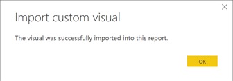

A new icon, bearing the Frontline Solvers logo is added under Visualizations.

Now we are ready to upload our data to Power BI. Click Get Data – More – Text/CSV, then click Connect.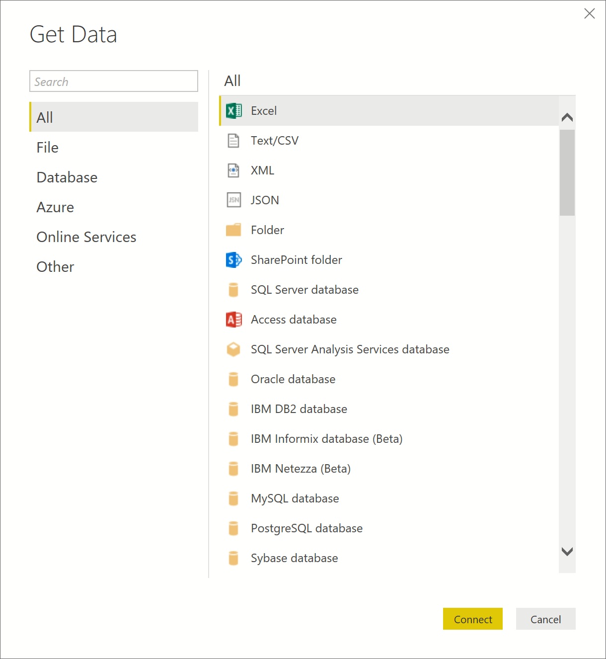

Navigate to the location of your data file(s), select the appropriate file(s) and then click Open. For simplicity's sake, the data for Power BI has been included within one file, ProductMixData.txt, however, all three data files could have been used.

Select the Data table on the Navigator window, then click Load. (Repeat these steps for each required data file.)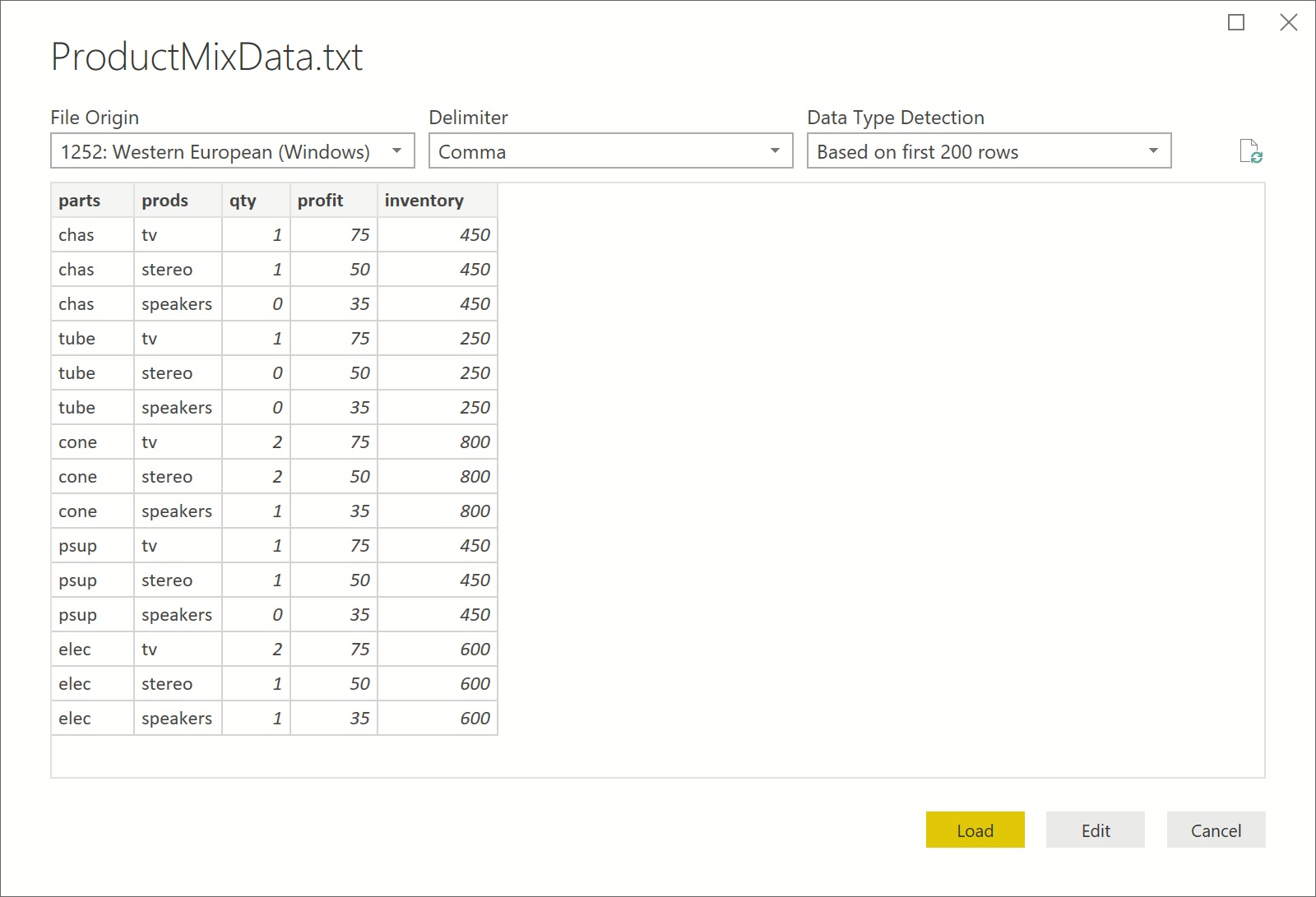

Multiple data fields are added beneath "Fields". These are our data fields.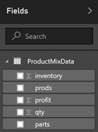

Select the Solver icon in Visualizations and notice new data "wells" appearing below. These "data wells" were created by the parts_data, profit_data and invent_data data sources.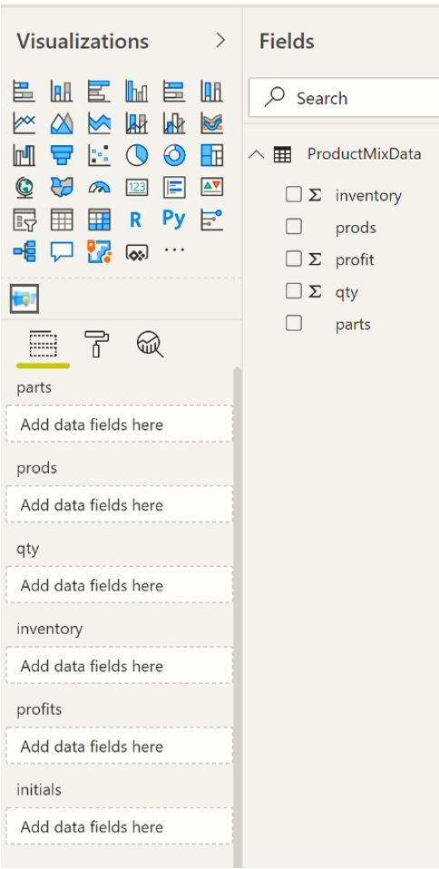

Drag the data fields into the data wells according to the following table.

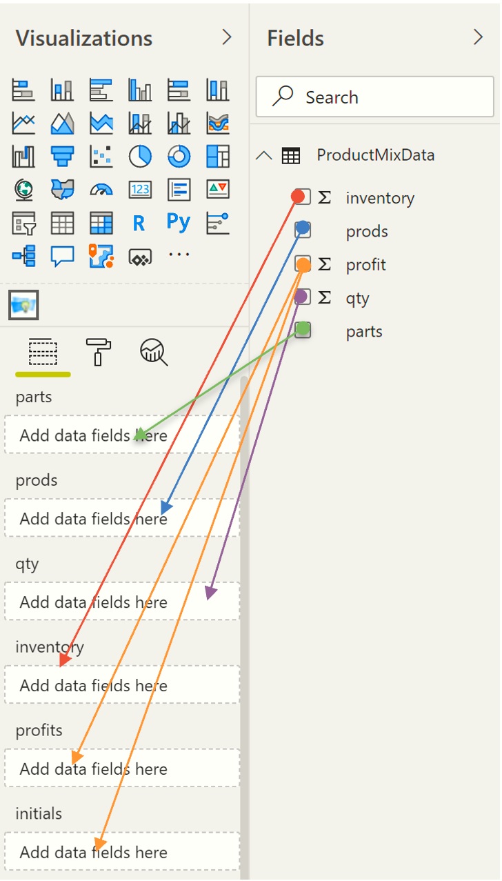
Afterwards, your task pane should match the following screenshot.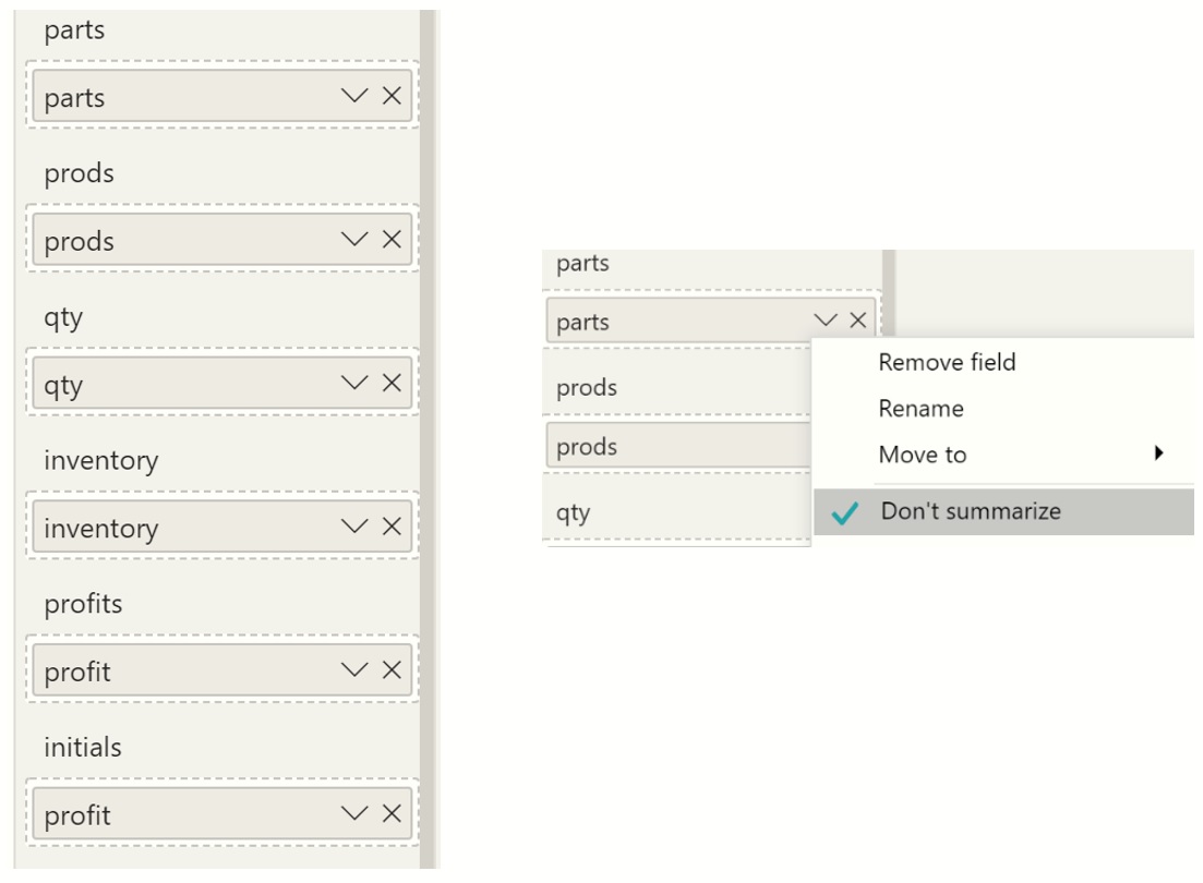

Immediately, the RASON model is submitted to the RASON Server, the model is solved and the final variable values are imported back into Power BI.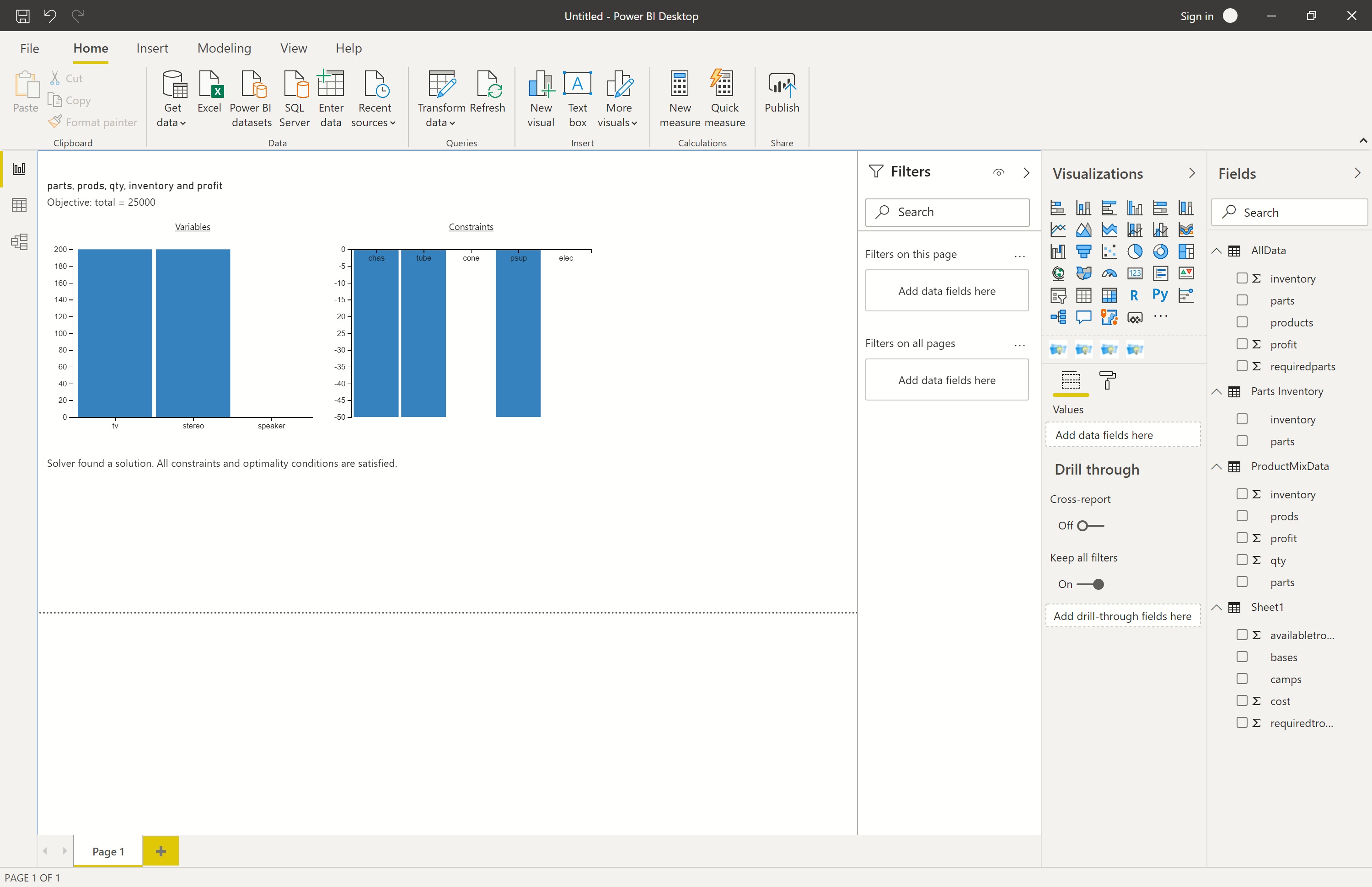

At the bottom of the custom visual, we find Solver’s result message: Solver found a solution. All constraints and optimality conditions are satisfied. Recall that since we are solving a linear model, this message indicates that Solver has found the globally optimal solution: There is no other solution satisfying the constraints that has a better value for the objective. For more information on this Solver result, please see the chapter “Solver Results Messages” within the Frontline Solvers Reference Guide.

In the first chart, we see that final variable values are: Var1 (LCD TV) equal to 200, Var2 (Stereo) equal to 200 and Var3 (Speakers) equal to 0. These variable values result in an objective function value equal to $25,000. In the chart to the right, we see the final constraint values are: Con1 (number of Chassis used) = 400, Con2 (number of LCD Screens used) = 200, Con3 (number of Speakers used) = 800, Con4 (number of Power Supplies used) = 400 and Con5 (number of Electronics used) = 600.

Advanced Settings

Recall from the examples above, once you click Create App -- Power BI, a dialog appears containing a checkbox for "Save Source".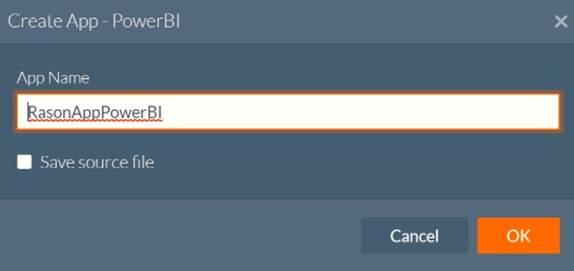

When this option is selected, a compressed file is created containing the pbiviz file. Save the contents of this file to a desired location. This file will contain the source code for the custom visual.

You will find the type script file, visual.ts within the src folder. Users can manipulate this file to customize the look and feel of the custom visual, such as the face of the custom visual icon (within Visualizations), alter the RASON model, etc. For more information on customizing the visual.ts file, see this webpage.

Note: If the visual.ts file is altered, a new pbiviz package must be created. To do so, open a command prompt, change the directory to the root directory of the custom visual and enter “pbiviz package”, as shown in the screenshot below.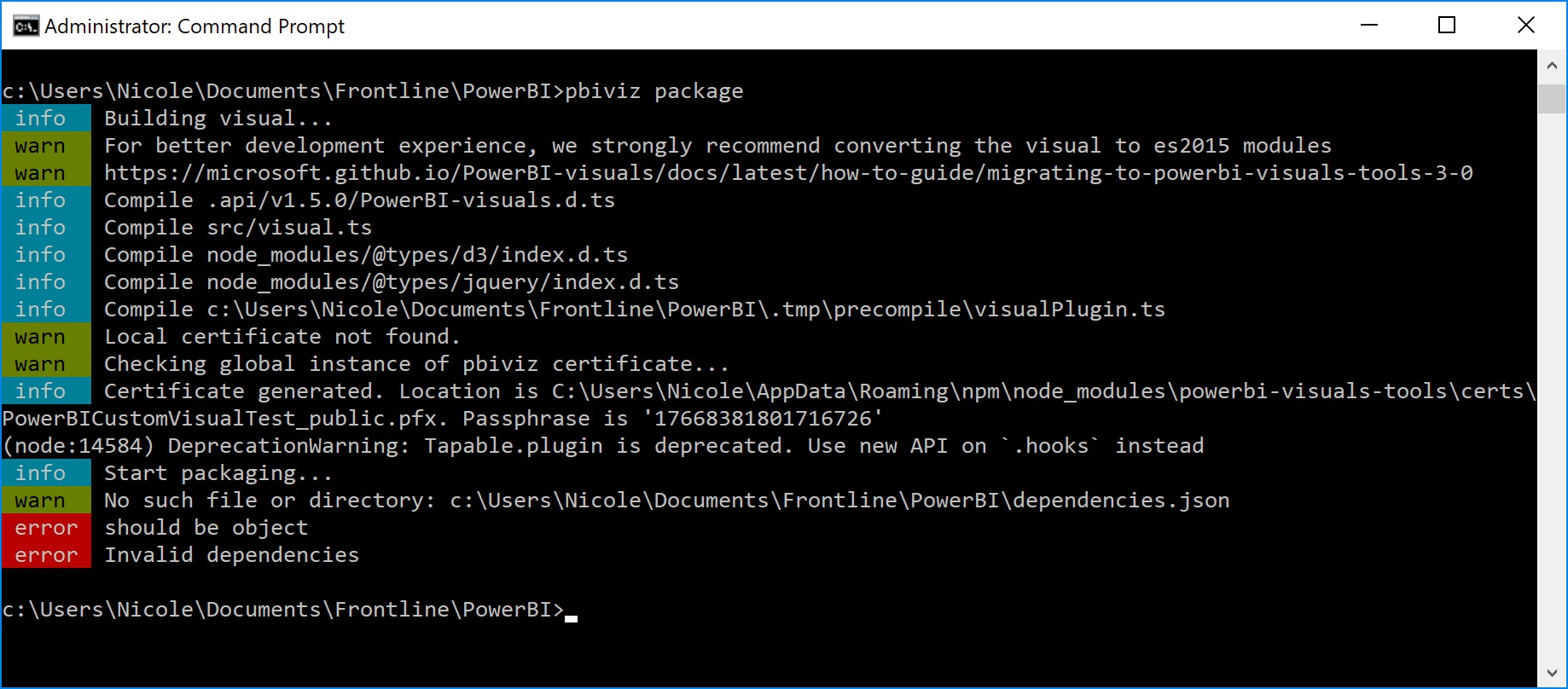

The new custom visual file (.pbiviz) will be saved to the Dist folder.